- 논문 : Learning to Adapt Structured Output Space for Semantic Segmentation
- 분류 : Domain Adaptation
- 읽는 배경 : Domain Adaptation 기본, Adversarial code의 좋은 예시
- 느낀점 :
- 참고 사이트 : Github page
AdaptSegNet
-
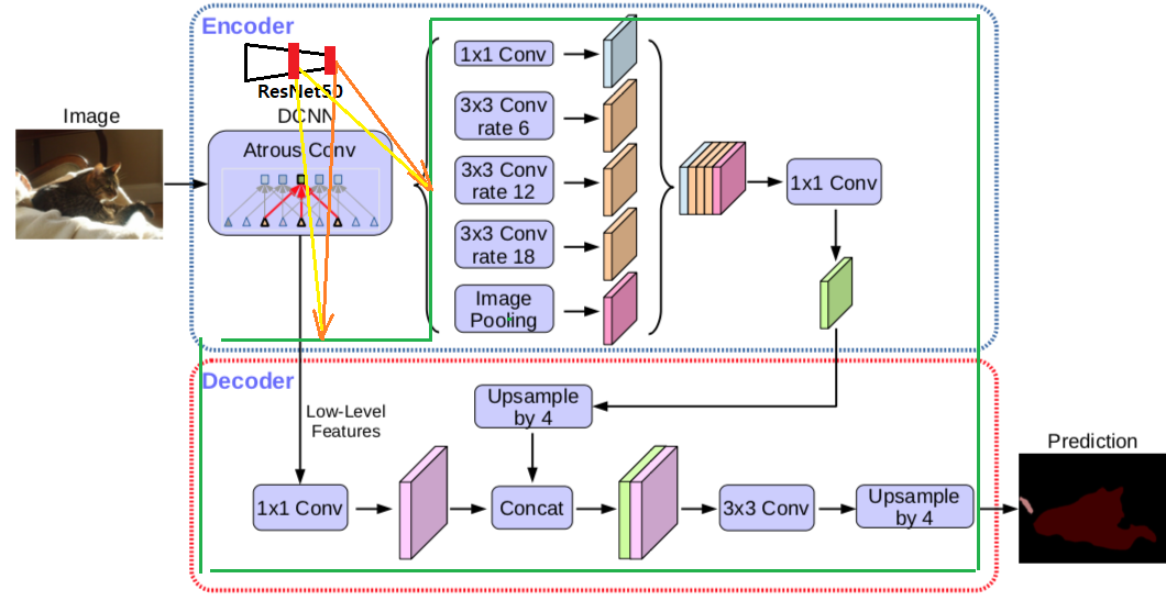
Deeplab V2를 사용했다고 한다. V2의 architecture 그림은 없으니 아래의 V3 architecture 그림 참조
-
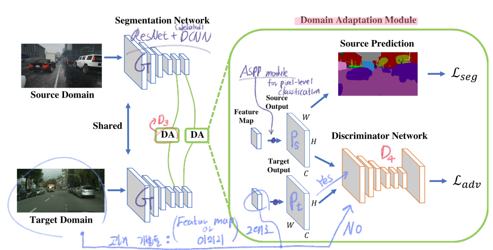
AdaptSegNet 전체 Architecture
-
코드를 통해 배운, 가장 정확한 학습과정 그림은 해당 나의 포스트 참조.
1. Conclusion, Abstract
- DA semantic segmentation Task를 풀기 위해, adversarial learning method을 사용한다.
- 방법1 : Adversarial learning을 사용한다. in the output space(last feature map, not interval feature map)
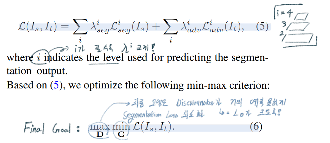
- 방법2 : 위의 그림과 같이 a multi-level에 대해서 adversarial network 을 사용한다. multi-level을 어떻게 사용하는지에 대해서는 위의 Deeplab V3 architecture를 참조할 것.
- 방법1의 Motivation : 아래 그림과 같이, 이미지 사이에는 많은 차이가 있지만, CNN을 모두 통과하고 나온 Output feature map은 비슷할 것이다.
- 따러서 Sementic segmentation의 예측결과 output을 사용하여, Adversarial DA과정을 진행함으로써, 좀더 효과적으로 scene layout과 local contect를 align할 수 있다.
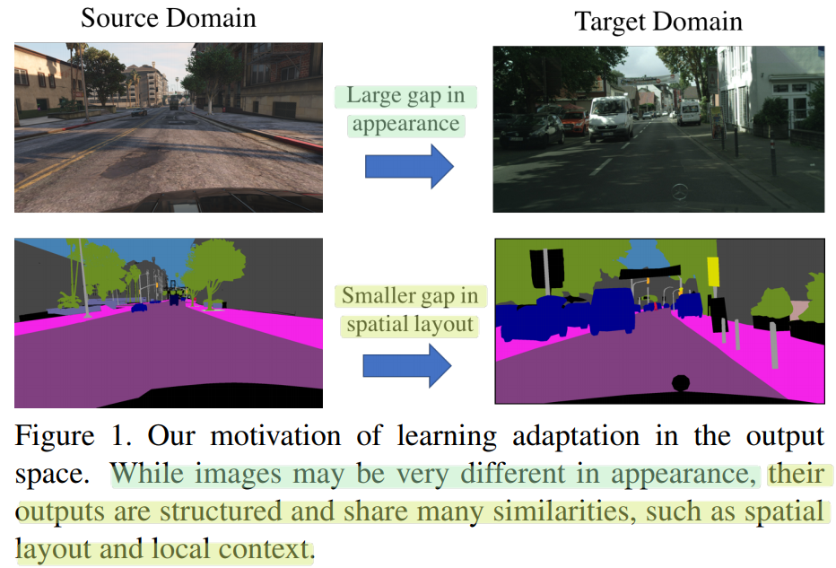
- 따러서 Sementic segmentation의 예측결과 output을 사용하여, Adversarial DA과정을 진행함으로써, 좀더 효과적으로 scene layout과 local contect를 align할 수 있다.
2. Instruction, Relative work
- pass
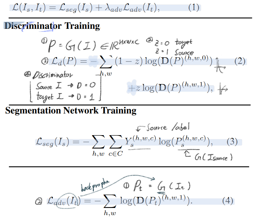
3. Method
- the discriminator D_i (level i): source 이미지로 부터온 prediction Ps인지 Target, 이미지로 부터온 prediction Pt인지 구별한다.
- target prediction에 대한 Adversarial loss를 적용해서, G(Generator=Feature encoder)가 similar segmentation distribution를 생성하게 만든다.
- Output Space Adaptation에 대한 Motivation
- 과거의 Adversarial 방법들은, 그냥 feature space(맨 위 이미지에서 빨간색 부분=complex representations)를 사용해서 Adversarial learning을 적용했다.
- 반면에, segmentation outputs(맨위 이미지에서, hard labeling 작업 이전의 최종 예측 결과값)은low-dimension이지만 rich information을 담고 있다.
- 우리의 직관으로 이미지가 source이든 target이든 상관없이, segmentation outputs은 굉장히 강한 유사성을 가지고 있을 것이다.
- 따라서 우리는 이러한 직관과 성질을 이용해서, low-dimensional softmax outputs을 사용한 Adversarial Learning을 사용한다.
- Single-level Adversarial Learning: 아래 수식들에 대해서 간단히 적어보자
- Total Loss
- Discriminator Loss: Discriminator 만들기
- Sementic segmentation prediction network
- Adversarial Loss: Generator(prediction network)가 target 이미지에 대해서도 비슷한 출력이 나오게 만든다
- Multi-level Adversarial Learning
- Discriminator는 feature level마다 서로 다른 Discriminator를 사용한다
- i level feature map에 대해서 ASPP module(pixel-level classification model)을 통과시키고 나온 output을 위 이미지의 (2),(3),(4)를 적용한다.
- Network Architecture and Training
- Discriminator
- all fully-convolutional layers, convolution layers with kernel 4 × 4 and stride of 2, channel number is {64, 128, 256, 512, 1},
- leaky ReLU parameterized by 0.2
- do not use any batch-normalization layers: small batch size를 놓고 각 source batch, target batch 번갈아가면서 사용했기 때문이다.
- Segmentation Network
- e DeepLab-v2 [2] framework with ResNet-101 [11] model
- modify the stride of the last two convolution layers from 2 to 1 함으로써, 최종결과가 이미지 H,W 각각이 H/8, W/8이 되도록 만들었다.
- an up-sampling layer along with the softmax output
- Multi-level Adaptation Model
- we extract feature maps from the conv4 layer and add an ASPP module as the auxiliary classifier
- In this paper, we use two levels.
- 위 그림을 보면 이해가 쉽니다.
- Network Training(학습 과정)
- (Segmentation Network와 Discriminators를 효율적으로 동시에 학습시킨다.)
- 위의 Segmentation Network에 Source 이미지를 넣어서 the output Ps를 생성한다.
- L_seg를 계산해서 Segmentation Network를 Optimize한다.
- Segmentation Network에 Target 이미지를 넣어서 the output Pt를 생성한다.
- Optimizing L_d in (2). 위에서 만든 Ps, Pt를 discriminator에 넣고 학습시킨다.
- Adversarial Learning : Pt 만을 이용해서 the adversarial loss를 계산하여, Segmentation Network를 Adaptation 시킨다.
- Hardware
- a single Titan X GPU with 12 GB memory
- the segmentation network
- Stochastic Gradient Descent (SGD) optimizer
- momentum is 0.9 and the weight decay is 5×10⁻⁴
- initial learning rate is set as 2.5×10⁻⁴
- the discriminator
- Adam optimizer
- learning rate as 10−4 and the same polynomial decay
- The momentum is set as 0.9 and 0.99
- Discriminator
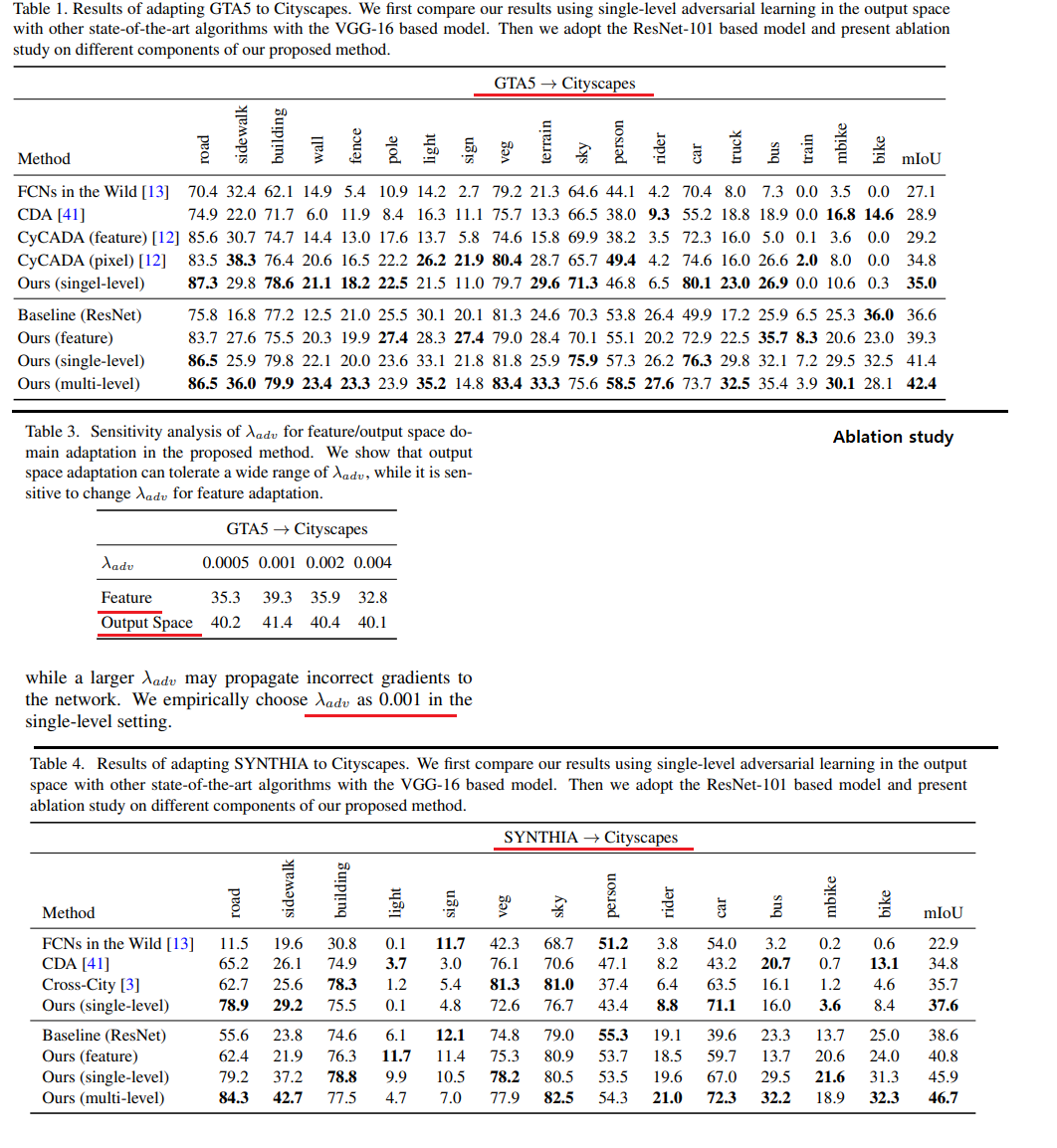
4. Results
- 성능 결과 및 Ablation study에 대한 내용은 Pass