[Algorithm] Key summary in preparation for coding interview
Python
- mutable vs Immutable [post1]
- import copy
- 메모리 공유 (1) =
- 딕,리스트 내부 딕 리스트는 메모리 공유 (2) .copy(), copy.copy(), [:]
- 딕,리스트 내부 딕 리스트까지 메모리 재할당(3) copy.deepcopy()
- Initializing a two-dim list: a = [ [0]*3 for i in range(3)]
- collections.deque: from collection import deque / q = deque([1,2,4,]) / q.append() / q.appendleft() / q.pop() / q.popleft()
- heapq: import heepq / heepq.heeppush(simple_list, 7) / heepq.heeppop(simple_list) / print(heaps[0]) / heapq.heapify(simple_list2)
- PriorityQueue: from queue import PriorityQueue / que = PriorityQueue(), que.put(k), que.get(). que.put((k, v)), que.get()[1]
- bisect: from bisect import bisect_left, bisect_right / bisect_right(list, value)
- collections.namedtuple
1. Recursion
- recursive function: a function calls itself.
- Base case: to stop the recursion
- Recursive case: where the function calls on itself
- Examples
- Easy: Factorial, Fibonacci number, Euclid method
- Hard: Towers of Hanoi, Maze, Cells in a Blob, N-Queens, Permutation
- Any problem solved recursively can also be solved through the use of iteration.
- 🪡 Binary search
- Finding a needed item from a sorted list, from the right or left. [logN]
- left right valuable → calculate middle and use it → break when (left≥right)
- from bisect import bisect_left, bisect_right / print(bisect_left(simpe_list, value))
- 🪡 Backtracking: (1) visit recursion (2) non-promising:fail / success:return.
- 🪡 State-space tree
2. Sort
- Selection sort
- Find the largest value in the list.
- Bubble sort
- left to right. Push back a larger one among 2 items. x N times
- Insertion sort
- left to right. The item finds its position in the its-left list.
- Merge sort
- not in-place
- divide and conquer
- mergesort(left) / mergesort(right) / merge
- Quick sort
- in-place
- pivot
- From the left, find an item smaller than the pivot.
From the right, find an item larger than the pivot.
- Heap sort
- in-place
- Max heap / Min heap / complete binary trees / Min-heapify: parent <= two children
- Main operation:
- Build heap: From non-leaf (internal) node, apply max-heapify.
- Insert: from bottom to top
- Delete: Delete top node. Last leaf node is placed on the top. Change the top with a smaller child
3. Search tree
- Linked structure: (1) Key(data) / (2,3) left+right children addresses / (4 optional) parent address
- Tree traversal (A - B, C - D E F G)
- Recursively: Inorder(left root right, DBEAFCG) / Preorder(root left right, ABDECFG) / Postorder (left right root, DEBFGCA)
- Binary search tree (=ordered tree)
- Definition: Internal nodes each store a key greater(≥) than all the keys in the node’s left subtree and less(≤) than those in its right subtree.
- (oper1) Search: O(hight=logN), min(leftmost), max(rightmost), Successor, Predecessor
- (oper2) Insert: O(hight=logN), Just need to find empty leaf.
- (oper3) Delete: If a deleted node has 0 or 1 child, no problem. But if 2 children, find successor
- Weakness: worst-case → O(N) → Keep balanced → red-black tree
- Red-black tree
- It is a kind of Binary search tree.
- Additional properties
- Every node is either red or black.
- NIL nodes are black.
- Red can not exist consecutively
- Example image, where 'h' is hight to NIL and 'bh' is the number of black nodes to NIL
- Key operation for search, insert, and delet: rotation
4. Hasing
- Hash table: Key and value
- Solutions of Collision:
- Chaining (linked list): worst-case → value unbalance problem
- Open addressing (Finding other empty space)
- linear probing: h(key) + i. Clustering problem
- quadratic probing: h(key) + i^2
- double hashing: use two different hash functions
- A critical problem of the above methods is the difficulty to delete & search.
- Good hash function is an almost random distribution function.
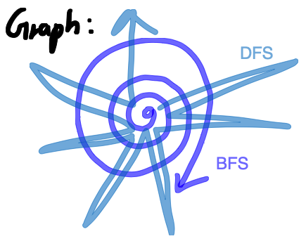
5. Graph - DFS,BFS
- Node, Edge, and adjacency matrix.
- Graph traversal [Reference image]
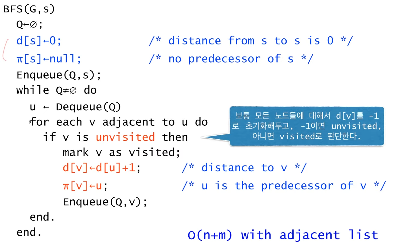
- BFS (Breadth-First Search)
- Queue: [pseudo code] (1) While queue is not empty (2) Remove a node v (3) For each unchecked neighbor w_s of v (4) Insert w into the queue and check it.
- Shortest path [pseudo code]: Needed valuables are d (distance) and π (predecessor, previous node).
- Note: Queue에 들어가는건 이미 방문한 node. 나중에 pop 할시, 그 노드에 인접한 것을 탐색한다.
- DFS (Depth-First Search)
- Recursive: [pseudo code] (1) DFS(G,v) (2) Check v (3) For each adjacent nodes w_s (4) If unchecked w, DFS(G,w)
- Note: 한 노드에 방문후, 인접한 노드를 recursively 호출
6. Graph2 - Minimum spanning tree
- Node, Edge, Weight(cost) → To connect all nodes, select minimum edges with minimum cost.
- Properties of MST: (1) non unique solution (2) non-cycle (3) edges of solutions can represent tree-structure (4) # edges = 1-#nodes
- Notations
- Goal: Finding safe {edges} = A = one MST solution
- Prerequisite: (1) Cut: 2subset S, V-S of nodes (2) Cross: edge cross 2subset (3) Respect: no cross edges in A
- Fact: If A is a subset of MST, the lightest edge, among edges cross the cut, respect A.
- Note: subset은 여러개가 될 수 있다. 새로운 edge를 고를때 연결된 node들이 이미 set을 이루고 있다면 cycle을 만드는 것이다.
- Kruskal algorithm
- Method: Sorted edges are sequentially selected, unless the edge makes a cycle, untill #nodes-1 == #edges.
- Proof: Sorting = the lightest edge / no cycle edge = Cross edge
- Key: checking whether a cycle exists. (1) Connected nodes represent a subset, e.g. [{a},{b,c,f},{e},{g,h}] (2) Using linked list, check wheter the root is same.
- Prim algorithm
- Method: From a random node, select the lightest cross-edge.
- Key: finding cross-edge: nodes in subset V-S need to contain two valuable, key and pie. ‘key’ is the lightest weight connecting with nodes in S. ‘pie’ is the connected node in S.
- Details: (1) Among nodes in V-S, find a node with the lightest ‘key’ value. (2) the node is inserted into S, nodes in V-S connected to the node update the value of ‘key’ and ‘pip’.
- Addition: Methods(1) needs to use Priority Queue (= min-heap, max-heap), so that the MST whole complexity is changed from O(n^2) to O(NlogN).
7. Shortest path
- Note: Path is different from Tree. MST is to find a tree with minimum cost. Dijkstra aims to find a path with minimum cost in a directed graph.
- Notations
- Properties: (1) sub-path inside the lightest path is also the lightest. (2) No-cycle
- Variables: (1) d[node]: initialized ‘inf’, distance from the start node s. (2) π[node]: predecessor
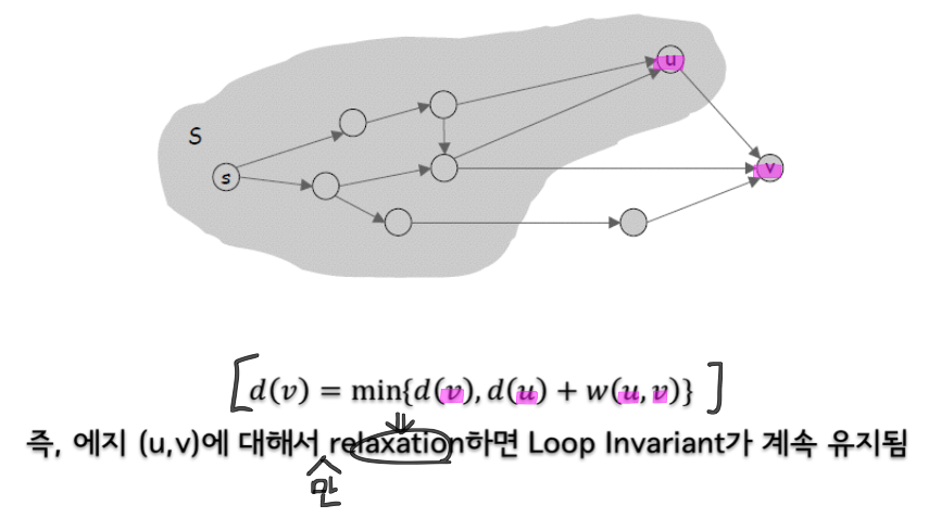
- Basic operation: Relaxation (if finding a better path, update d and π)
- Bellman-ford algorithm
- If there are negative weights.
- [Example image] O(n*m) is too big. Thus, Dijkstra does not depend on m!
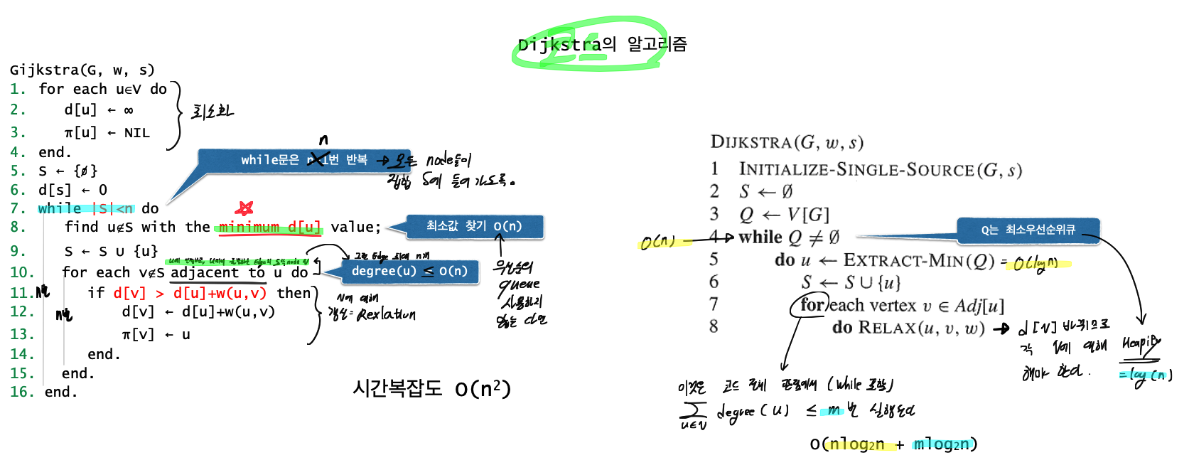
- Dijkstra algorithm
- Assume that there is no negative weight. | Checked node is never checked again.
- In a set of unchecked nodes, a node with minimum d[node] must be the node for the next step. [reference image]
- [Pseudo code]
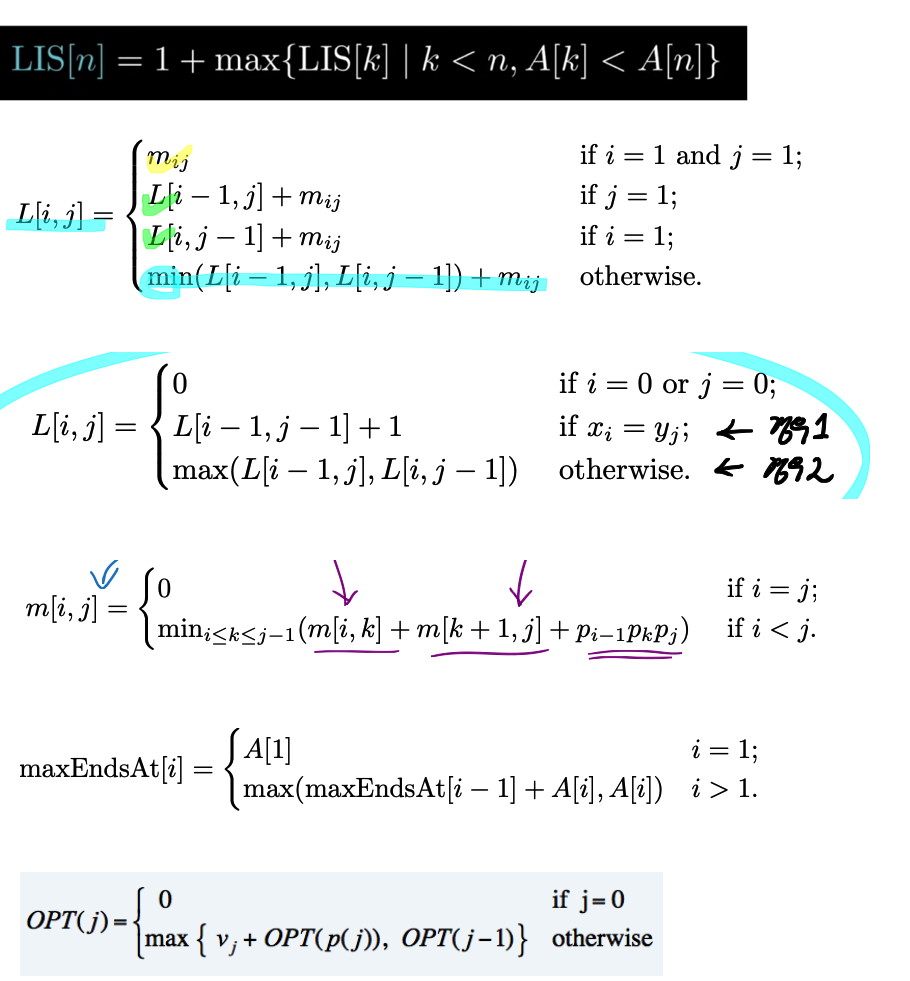
8. Dynamic programming
- Key
- Building recursive equation.[Example image]
- Problems can divide into sub-problems. The optimal solution of sub-problem is a part of the Optimal solution to the entire problem.
- Memoization (For overlapped sub-problem)
- Bottom-up